How to make a Gantt chart in Excel

This step-by-step Excel Gantt chart tutorial will show you how to make professional Gantt charts using Excel and PowerPoint.

Options for making a Gantt chart

Microsoft Excel has a Bar chart feature that can be formatted to make an Excel Gantt chart. If you need to create and update a Gantt chart for recurring communications to clients and executives, it may be simpler and faster to create it in PowerPoint.

On this page, you can find each of these two options documented in separate sections. First, we will give you step-by-step instructions for making a Gantt chart in Excel by starting with a Bar chart. Then, we will also show you how to instantly create an executive Gantt chart in PowerPoint by pasting or importing data from an .xls file.

Which tutorial would you like to see?

How to make a Gantt chart in Excel

1. List your project schedule in an Excel table.

1. Break down the entire project into chunks of work, or phases. These will be called project tasks and they will form the basis of your Gantt chart.

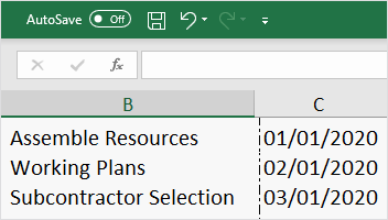
2. In Excel 2013, 2016 and 2019, enter your data by listing the Start Date and Finish Date of each task, along with their duration (count of days required to complete that task). Make sure to include a brief description for each task, and then sort them in order, by placing the earliest start date first and the latest date last, as shown in the image below.

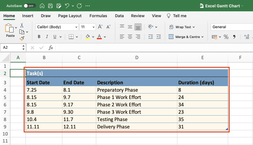
In this tutorial, we will convert this table into an Excel Gantt chart and then into a PowerPoint Gantt chart. Read on to learn how.

2. Begin making your Excel Gantt by setting it up as a Stacked Bar Chart.

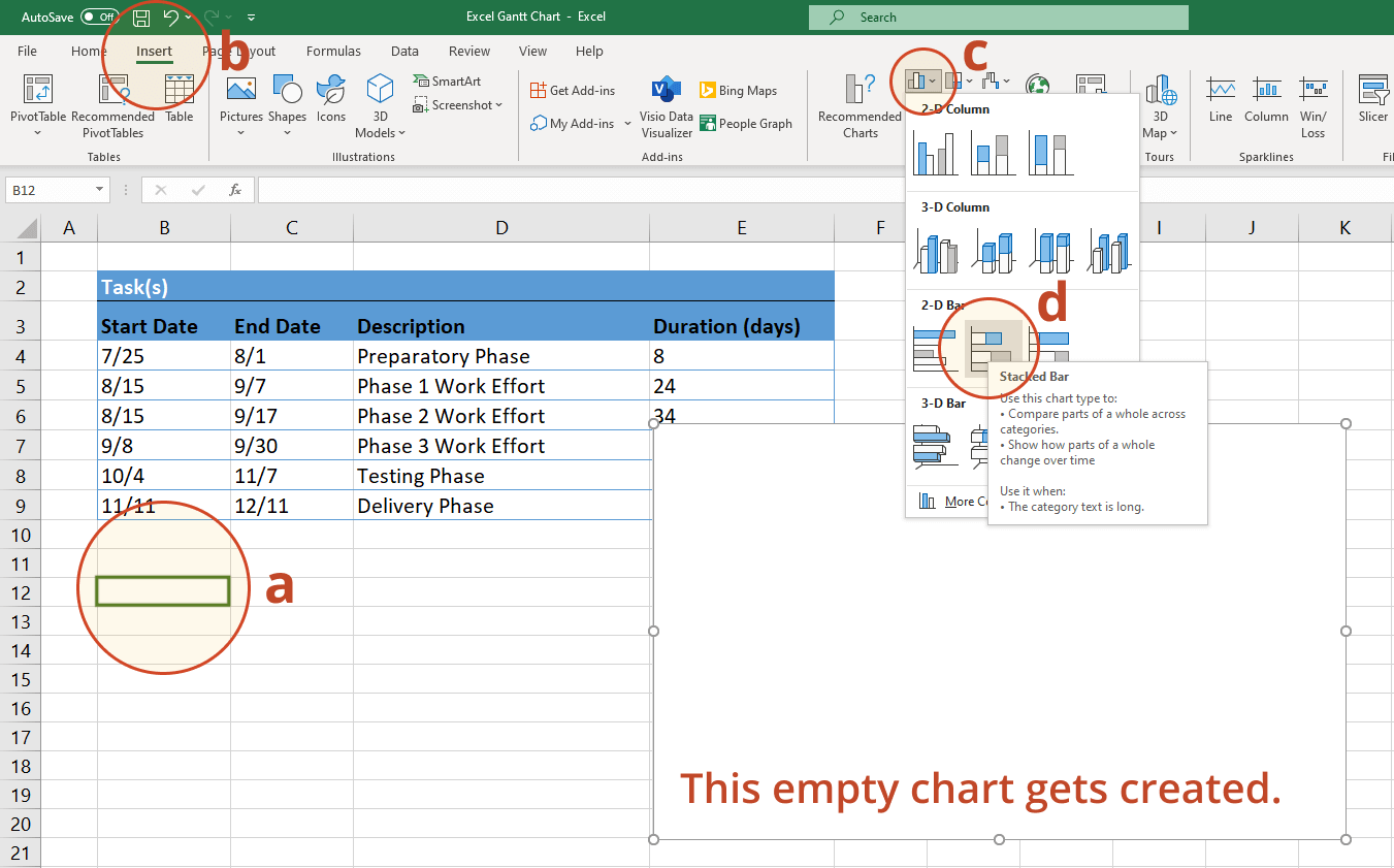
1. Within the same worksheet that your Excel table is on, click in any blank cell.

2. From the Excel ribbon, select the INSERT tab.

3. In the Charts section of the ribbon, drop down the Bar Chart selection menu.

4. Then select Stacked Bar, which will insert a large blank white chart space onto your Excel worksheet (do not select 100% Stacked Bar).

   

3. Add the start dates of your tasks to the Gantt chart.

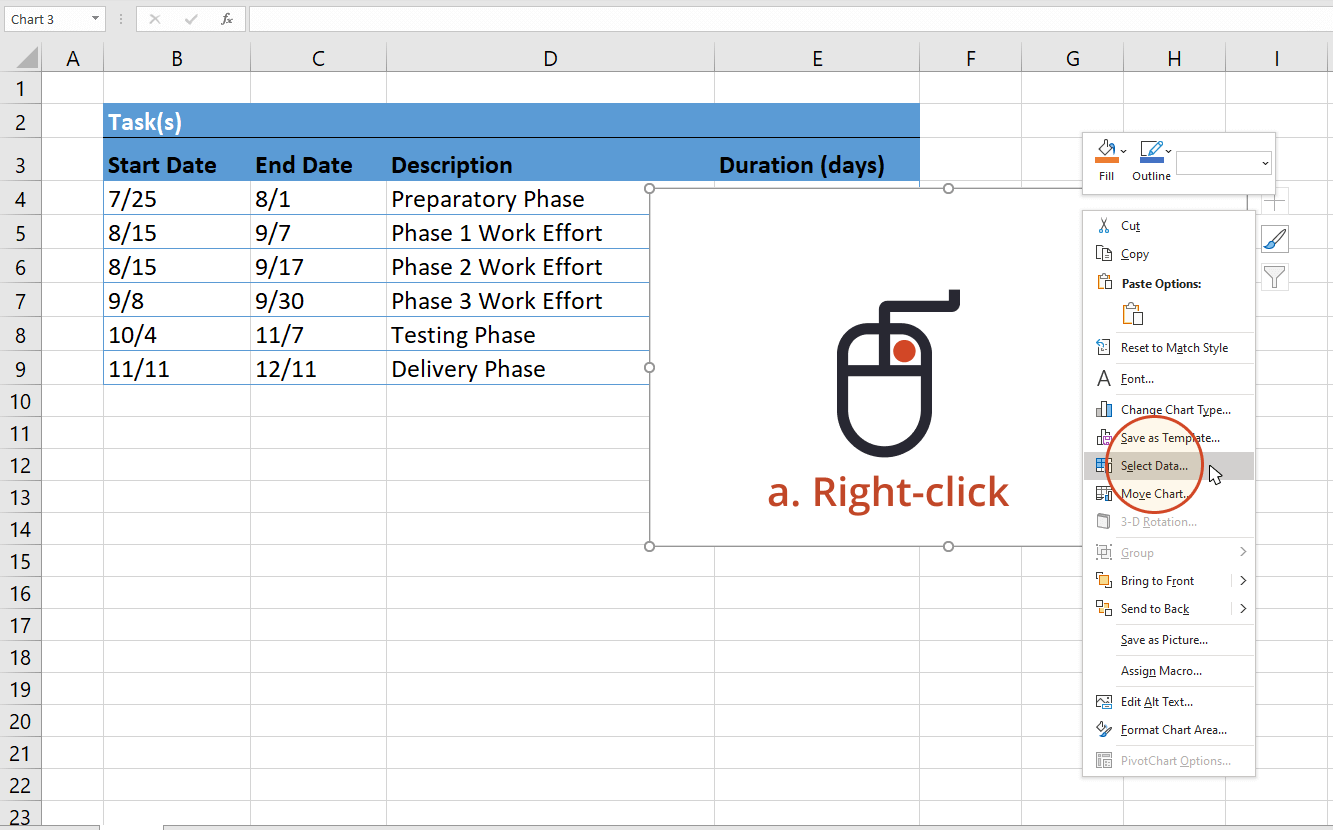
1. Right-click the white chart space and click Select Data to bring up Excel's Select Data Source window.

   

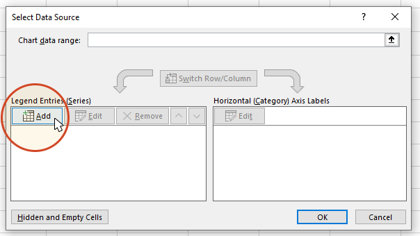
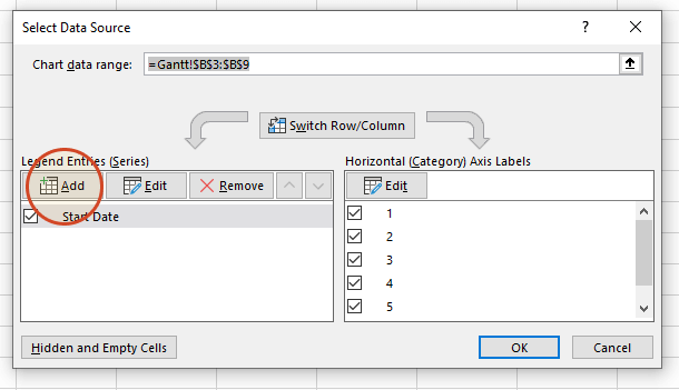
2. On the left side of Excel's Data Source window, you will see a table named Legend Entries (Series). Click on the Add button to bring up Excel's Edit Series window where you will begin adding the task data to your Gantt chart.

   

3. Now we're going to add your task data.

   i. First, we need to name the data (Series) we will be entering. Click and place your cursor in the empty field under the title Series name, then click on the column header that reads Start Date in your table.

   ii. Staying in the Edit Series window, move down to Series value. This is where you will enter your Task start dates. It is easy to do. To the right of the Series values field you will see an icon with an arrow pointing up.

   

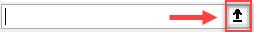
   Click on the icon and Excel will open a smaller Edit Series window. Now simply click the first start date in your task table and drag your mouse down to the last start date. This highlights all of the start dates for your tasks and inputs them into your Gantt chart. Make sure you have not mistakenly highlighted the header or any extra cells.

   

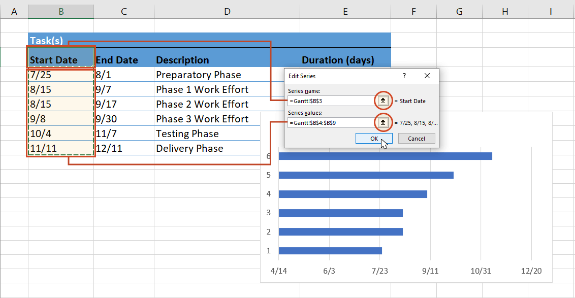
   iii. When finished, click on the arrow icon again , which will return you to the previous window called Edit Series. Once here, click OK. Your Gantt should now look like this:

   

4. Add the durations of your tasks to the Gantt chart.

1. Stay in the Select Data Source window and re-click the Add button to bring up Excel's Edit Series window. Here is where you will add the duration data to your Gantt chart.

   

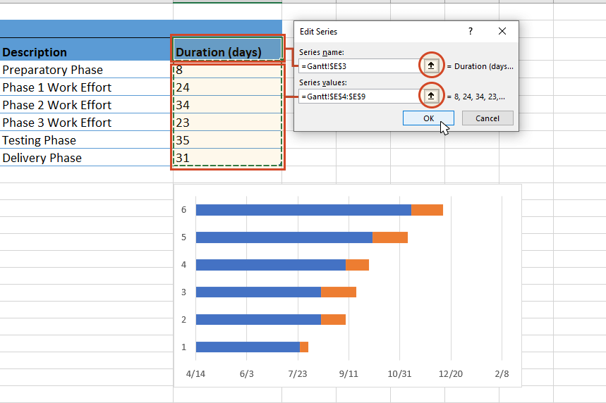
2. In the Edit Series window, click in the empty field under the title Series Name and then in your task table again, on the column header that reads Duration.

   

3. Staying in the Edit Series window, move down to Series value and click once more on the spreadsheet icon with a black arrow on it (called Edit Series Button) . Select your Duration data by clicking on the first duration in your project table, and drag your mouse down to the last duration so all durations are now highlighted.

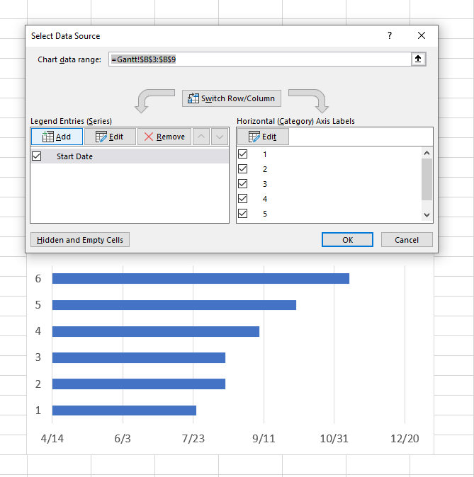
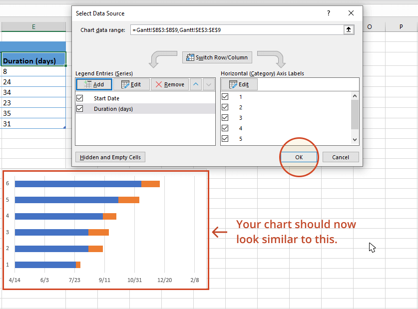
4. To exit, click again on the small spreadsheet icon with the black arrow, which will return you to the previous window. Select OK and you should now be back in the Select Data Source window. Click OK again to update your Gantt chart which should now look something like this:

5. Add the descriptions of your tasks to the Gantt chart.

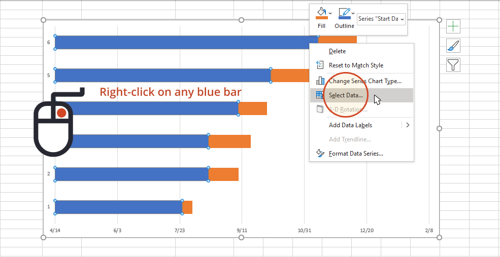
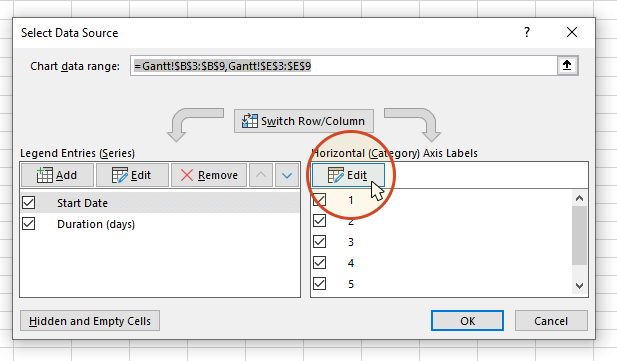
1. Right-click on one of the blue bars in the Gantt chart, then click on Select Data again to bring up the Select Data Source window.

   

2. On the right side of Excel's Data Source window, you will see a table named Horizontal (Category) Axis Labels. Select the Edit button to bring up a smaller Axis Label windows.

   

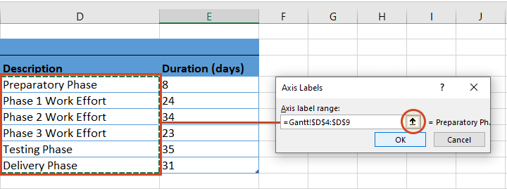
3. Again, click on the small spreadsheet icon. Then click on the first name of your tasks (in our example, the first task description is "Preparatory Phase") and select them all. Be careful not to include the name of the column itself. When you are done, exit this window by clicking on the small black arrow icon again.

   

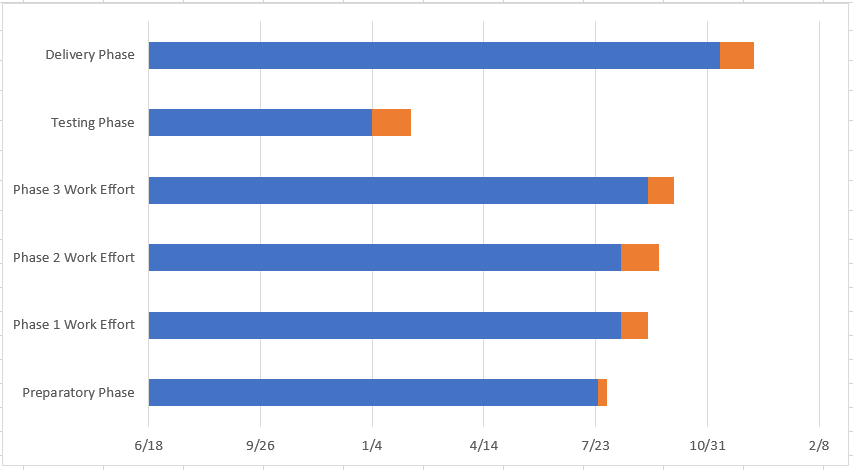
4. Click OK and then OK again to exit the Select Data Source window. Now your Gantt chart should have the correct task descriptions next to their respective bars, and should look something like this:

   

6. Format your chart so it looks like a Gantt chart.

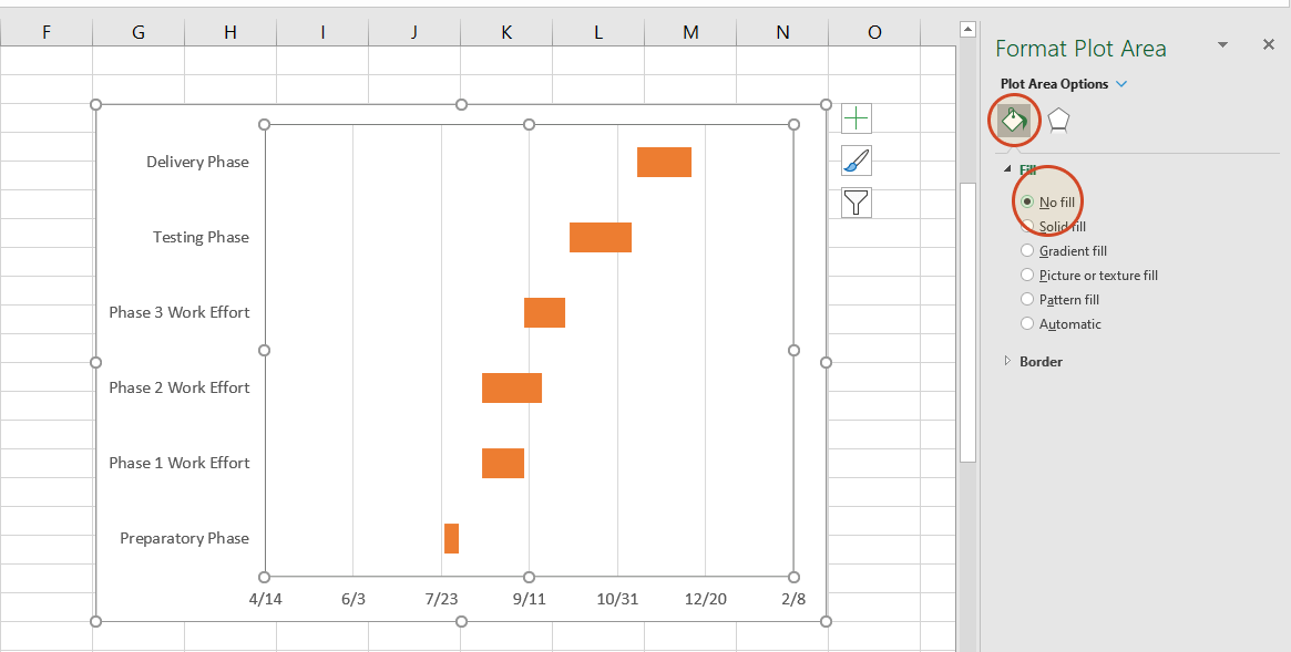
Up to this point, you have really built a Stacked bar chart. Now we need to format it so it looks like a Gantt chart. To do that, we must make the blue parts of each task bar transparent so only the orange parts will be visible. These will become the tasks of your Gantt chart.

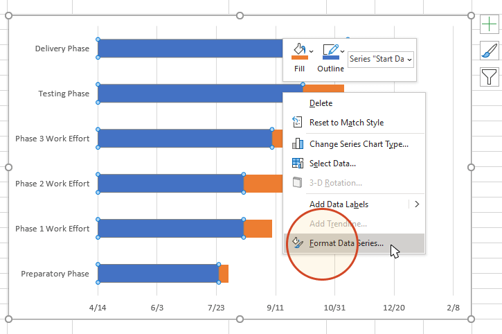
1. To select all of the task bars at once, click on the blue part of any bar in your Gantt chart, then right-click and select Format Data Series, which will bring up the Format Data Series window in Excel.

   

2. In the Format Data Series task pane, click on the Fill & Line icon (it looks like a paint can) to get the Fill & Line options. Under Fill, tick the No Fill radial button and, under Border, choose the No Line option. Don't close the Format Data Series task pane because you're going to use it in the next step.

   Your Gantt chart should now look like this:

   

3. You will probably notice that the tasks on your Gantt chart are listed in reverse, with the last task on top of the Gantt chart and the first task listed at the bottom. However, you can easily arrange them in counter direction in Excel.

   i. To do so, click on the list of tasks along the vertical axis of your Gantt chart. This will select them all and it will also open the Format Axis task pane.

   ii. Here, in the Format Axis task pane, click on the Bar Chat icon to expand out the Axis Options menu.

   iii. In the Format Axis task pane, under the header Axis Options and the sub-header Axis Position, tick the checkbox called Categories in reverse order.

   

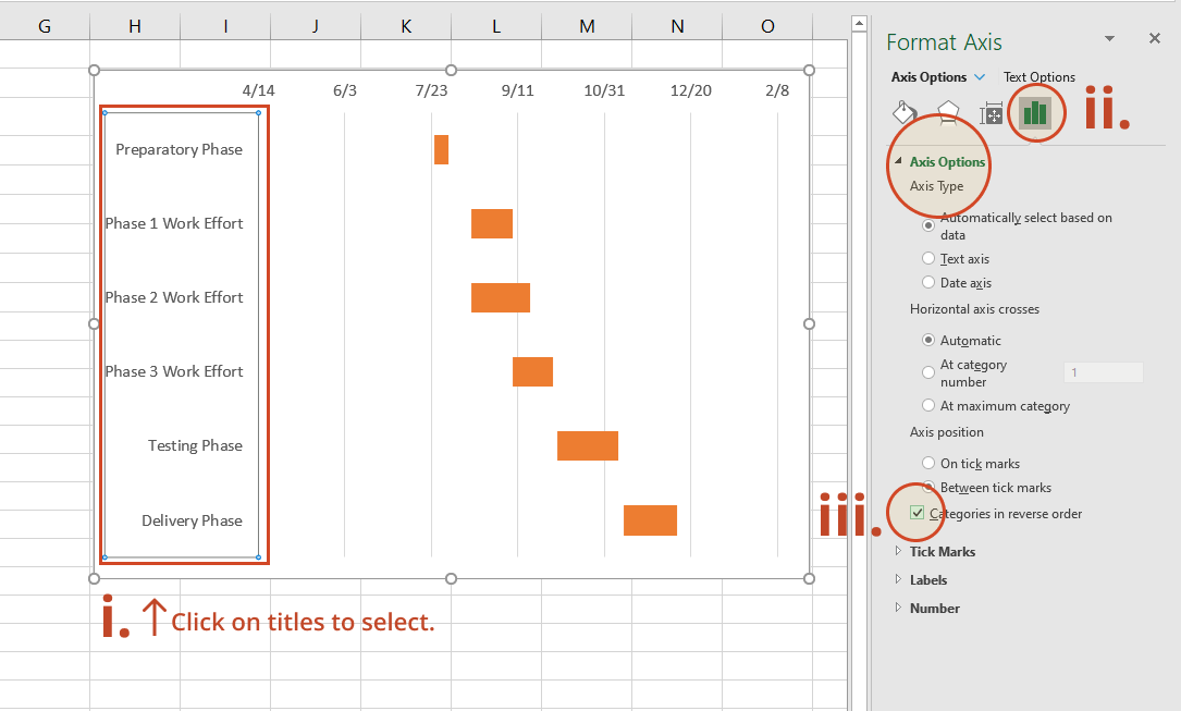
   You will notice that Excel not only arranged your tasks from first to last on your Gantt chart, but also moved the date markers from beneath to the top of the graphic. Now it is really starting to look more like a Gantt chart should.

7. Finish your Gantt chart with these styling tips.

Now that your Gantt chart is created, you can further style it to optimize its layout and legibility. Here are a few suggestions in this respect.

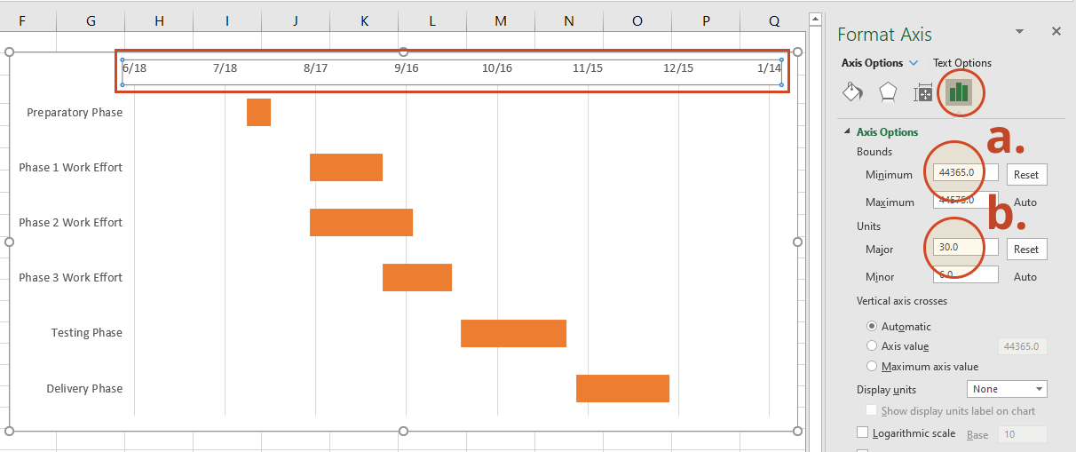
1. Reduce the white space on your Gantt chart

   Removing some of the blank white space where the blue bars used to be will bring your tasks a little closer to the vertical axis of your Gantt chart. To do this, click on any of the dates above the task bars to have all of them selected. Then, right-click and select Format Axis to bring up Excel's Axis Options window.

   In the Axis Options window, under the header called Bounds, note the current number for Minimum Bounds. It represents the left most boundary of your Gantt chart. Changing this number by making it larger will bring your tasks closer to the vertical axis of your Gantt chart. In our case, we changed the original number (which was 44300.0) to 44365.0. At any time, you can hit the reset button to restore the original settings. This gives you the opportunity to try several different settings until you find the one that makes your Gantt chart look best.

2. Adjust the density of the dates across the top of your Gantt chart

   In the same Axis Options window under the header Units, you can adjust the spacing between the dates listed at the top of the horizontal Axis. If you increase the Major unit number, Excel will enlarge the space between each date and, thus, lessen the number of dates your Gantt chart shows. Doing the opposite will reduce the space between each date and, therefore, create extra room for more dates onto your Gantt chart. In our case, we changed the original number from 20 to 30.

   

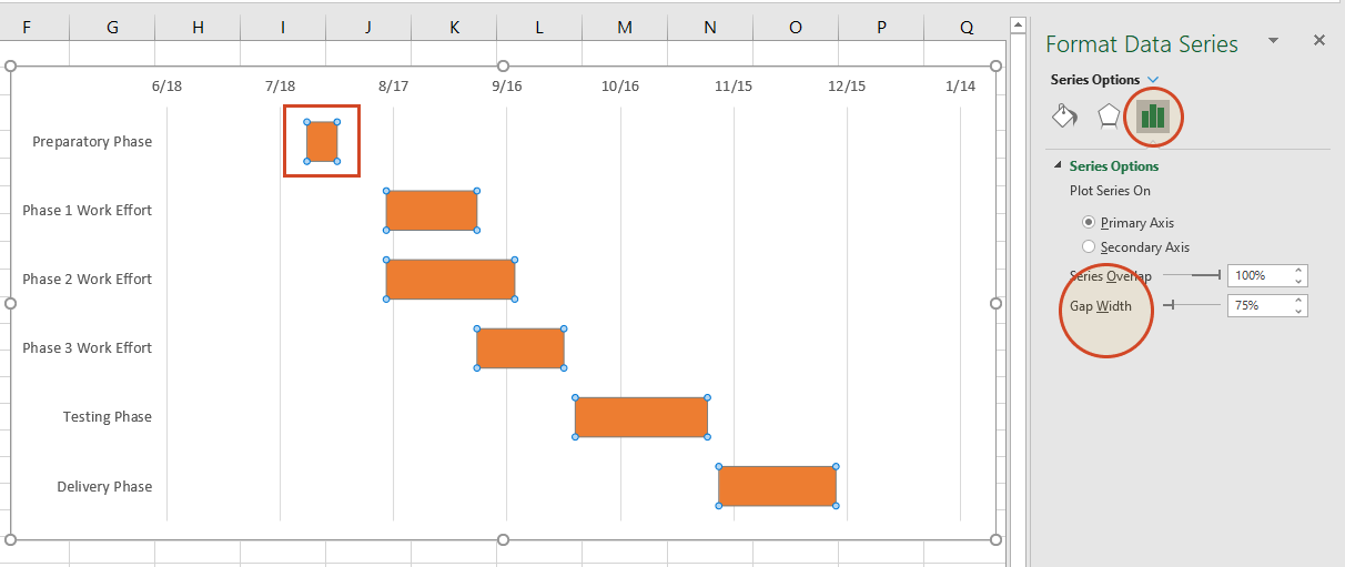
3. Make the task bars on your Gantt chart thicker

   Right-click on the first task bar and choose Format Data Series to open the Format Data Series control. Under the Series Options header, you will find the Gap Width control. Sliding it up or down will increase or reduce the size of the task bars on your Gantt chart. Play around until you find something that best works for you.

   

4. Customize task bars and chart area

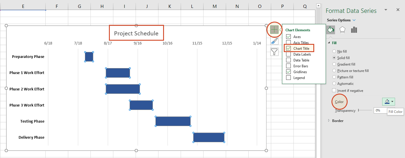
   As a finishing touch, you may want to add a title to your Gantt chart, change the color of the task bars or use another type of text font. In our case, we chose to:

   - recolor the chart bars from orange to a dark blue by double-clicking on any of the bars, going to the Fill & Line section of the Format Data Series pane on the right, and using the Fill color option menu;

   - use Bold font for the text of the task descriptions. If you want to do the same, simply click on the titles to select them all, and then press Ctrl + B;

   - add a title to the graphic by selecting the chart area, clicking on the “+” button in the upper right corner, and then ticking the box in front of Chart Title. This will insert a text box at the top of your Gantt in which you need to double-click in order to continue typing in the name for your visual.

   

Download Excel Gantt chart template file

Excel-Gantt-Chart-Template.xlsx

How to make a Gantt chart in PowerPoint

PowerPoint is a more graphical tool and a better choice for making Gantt charts that will be used in client and executive communications. Office Timeline is a PowerPoint add-in that makes and updates Gantt charts by importing or pasting from Excel.

You can copy-paste, import and refresh the data from your Excel tables in PowerPoint. In the steps below, we will demonstrate how to turn the Excel table you created above into a PowerPoint Gantt chart by using Office Timeline Pro+.

1. Open PowerPoint and paste your table into the Office Timeline wizard.

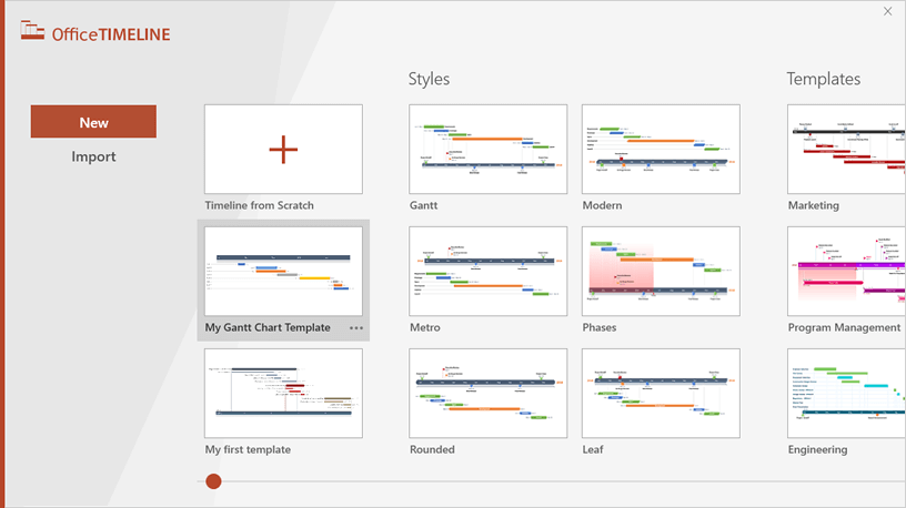
1. Inside PowerPoint, navigate to the Office Timeline Pro+ tab and click the New button.

   

   This will open a gallery that will allow you to choose a style or template for your Gantt chart.

   

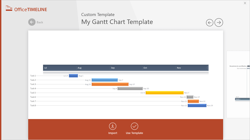
2. From the gallery, double-click any template or style to select it, and then click Use Template in the preview window to open the Data Entry Wizard. In this demonstration, we will be using a custom template which comes with sample data, but you can delete them. NOTE: If you prefer to import and refresh your Excel table, rather than copy-paste it, select Import.

   

3. Copy your project's details, including Start Date, End Date and Description, from the Excel table you made earlier. You can copy them all at once but be sure not to copy the title.

   

4. Now simply paste the data into PowerPoint using the Office Timeline Pro+ Paste button. Then, make any edits you wish (change colors or shapes, add or remove items, etc.) and click Create.

   

2. Your Excel table will be converted into a PowerPoint Gantt chart.

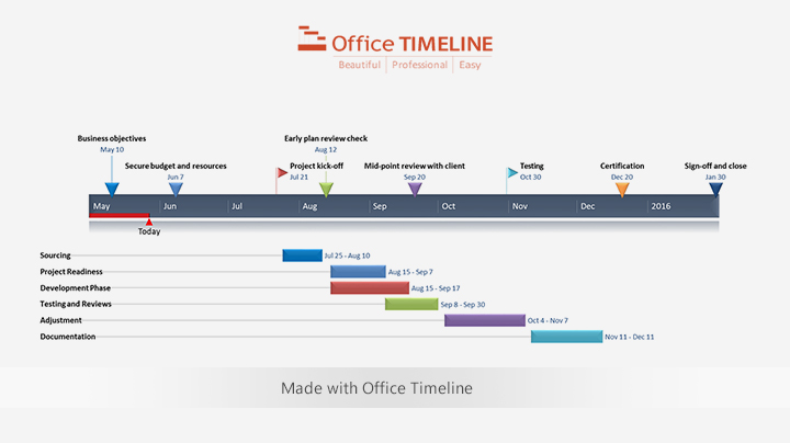
1. Depending on the style or template selected, you will have a Gantt chart that looks like this:

   

2. From here, you can easily customize the Gantt chart further, adding milestones, formatting fonts and colors, and adding various details like percent complete or notes. It is easy to do in Office Timeline. In our example, we used Office Timeline Pro+ to add milestones, move task titles and date texts, change shapes, and add percent complete.

   

Download PowerPoint Gantt chart template file

PowerPoint-Gantt-Chart-Template.pptx

FAQs about making Gantt charts in Excel

Here are the answers to the most frequently asked questions in relation to making Gantt charts in Microsoft Excel.

How do I create a Gantt chart template in Excel?

To create a Gantt chart in Excel that you can use as a template in the future, you need to do the following:

1. List your project data into a table with the following columns: Task description, Start date, End date, Duration.
2. Add a Stacked Bar Chart to your Excel spreadsheet using the Chart menu under the Insert tab.
3. Add the start and end dates of your tasks to your stacked bar chart.
4. Add the duration of your tasks to the graphic.
5. Add the task descriptions to your Excel stacked bar chart.
6. Format the stacked bar chart to make it look more like a Gantt chart by turning the blue segment of the bars transparent.
7. Improve the legibility of the Gantt chart by:
   • bringing the task bars closer to the vertical axis of the chart;
   • adjusting the density of the task dates;
   • thickening the task bars to reduce the white space.

Is there an Excel Gantt chart template?

As shown in the tutorial above, Excel doesn’t have any predefined Gantt chart templates per se, but it allows you to create a basic Gantt sample by manually formatting a stacked bar chart.

Alternatively, if you want to save time and make a Gantt chart faster, you can do so by importing or pasting your data from Excel into PowerPoint.

To better understand how you can do that, check out our short video below.

How to make a PowerPoint Gantt chart from Excel in under 60 seconds: